Graphing real polynomials | Year 12

01 / LEARN

Understand the idea.

Build a sketch from information you can justify

Start a polynomial sketch with its real zeros, their multiplicities and $P (0)$ . Label the corresponding intercepts. At an even-multiplicity root the curve touches the axis; at an odd-multiplicity root it crosses.

The leading term determines the far ends. Even degree sends both ends in the same direction; odd degree sends them in opposite directions. A positive leading coefficient gives a right end rising to positive infinity; a negative one reverses that direction.

Add enough detail without inventing features

Use the signs of factors to decide whether each interval lies above or below the axis. This checks that the crossings and touches fit together. Extra plotted points may refine the picture, but should not create unsupported intercepts.

When precise stationary points are needed, solve $P^{'} (x) = 0$ , find their ordinates and classify them using derivative signs or a conclusive second-derivative test. Otherwise show the justified qualitative shape without inventing exact coordinates.

02 / WORKED EXAMPLES

See the method in action.

EXAMPLE 01

A cubic with a double root

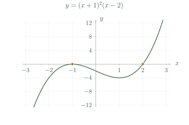
Sketch $P (x) = {(x + 1)}^{2} (x - 2)$ , showing roots, the y-intercept and end behaviour.

Graph of y=(x+1) squared times (x-2), with x from minus three to three and y from minus twelve to twelve. It touches the x axis at minus one, crosses at two, and has y intercept minus two.

Worked solution

1
Identify the intercepts on the horizontal axis.
$P (x) = 0 \Rightarrow x = - 1 (multiplicity 2), x = 2 (multiplicity 1) .$
The curve touches at $(- 1, 0)$ and crosses at $(2, 0)$ because of the root multiplicities.
2
Locate the vertical intercept.
$P (0) = {(0 + 1)}^{2} (0 - 2) = - 2.$
Substituting zero gives the point $(0, - 2)$ .
3
Set the end directions.
$\begin{aligned} P (x) & \sim x^{3}, \\ P (x) & \to - \infty & as x \to - \infty, \\ P (x) & \to \infty & as x \to \infty . \end{aligned}$
The leading term is a positive cubic.
4
Check signs and join the features smoothly.
$\begin{aligned} P (x) & < 0 & for x < 2, x \neq - 1, \\ P (x) & > 0 & for x > 2. \end{aligned}$
The squared factor is positive away from $- 1$ , so the other factor determines the sign. The touch at $- 1$ stays below the axis on both sides.

Answer

Touch at $(- 1, 0)$ ; cross at $(2, 0)$ ; pass through $(0, - 2)$ .

EXAMPLE 02

Stationary points when required

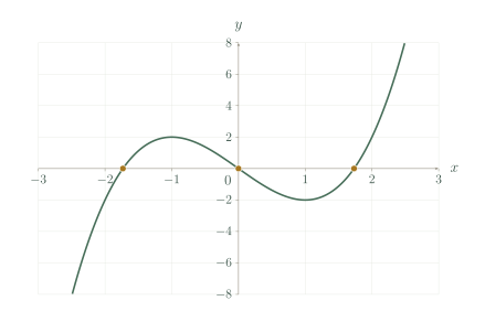
Find the stationary points of $P (x) = x^{3} - 3 x$ and identify their type.

Graph of y=x cubed minus 3x, shown on x from -3 to 3 and y from -8 to 8. The three original zero markers are at x=-square root of 3, zero, and square root of 3. No stationary-point answer labels have been added.

Worked solution

1
Find the stationary inputs.
$P^{'} (x) = 3 x^{2} - 3 = 3 (x - 1) (x + 1) = 0 \Rightarrow x = - 1, 1.$
A polynomial is differentiable everywhere, so stationary points occur at zeros of its derivative.
2
Find their ordinates.
$\begin{aligned} P (- 1) & = {(- 1)}^{3} - 3 (- 1) = 2, \\ P (1) & = 1 - 3 = - 2. \end{aligned}$
Stationary inputs must be substituted into the original function.
3
Classify using the second derivative.
$P^{''} (x) = 6 x, P^{''} (- 1) = - 6 < 0, P^{''} (1) = 6 > 0.$
A negative second derivative gives a local maximum and a positive one gives a local minimum.
4
State both stationary points.
$Local maximum (- 1, 2); local minimum (1, - 2) .$
The classifications are attached to points, rather than to input values alone.

Answer

Local maximum $(- 1, 2)$ ; local minimum $(1, - 2)$ .

03 / YOUR TURN

Try it yourself.

Check your understanding

What happens at each end of $y = - 3 x^{4} + 2 x - 1$ ?

Show answer & reasoning

Both ends go downwards.

The leading term is $- 3 x^{4}$ . Since $x^{4} \to \infty$ at both ends, $- 3 x^{4} \to - \infty$ at both ends; the lower-degree terms do not change this end behaviour.

Keep practising

6 worksheet questions · 15 marks

Open worksheet Worked solutions

Read the questions online

For $P (x) = x {(x - 2)}^{2}$ , state roots, multiplicities and end behaviour.
2 marks
Find the $y$ -intercept and end behaviour of $P (x) = - 2 (x + 1) (x - 3)$ .
2 marks
State the sign of ${(x + 1)}^{2} (x - 2)$ on the intervals separated by $- 1$ and $2$ .
2 marks
Write a monic quartic that touches the axis at $- 2$ and $1$ and has no other roots. Find its $y$ -intercept.
2 marks
Find the stationary points of $P (x) = x^{3} - 6 x^{2} + 9 x$ .
4 marks
Explain why a positive-leading cubic must have at least one real zero.
3 marks

Read the worked solutions

Equivalent correct methods earn the corresponding marks. Include units where asked.

For $P (x) = x {(x - 2)}^{2}$ , state roots, multiplicities and end behaviour.
2 marks
The leading term is $x^{3}$ and the factor powers give multiplicities.
$0$ simple/crosses; $2$ double/touches; left down, right up.
Find the $y$ -intercept and end behaviour of $P (x) = - 2 (x + 1) (x - 3)$ .
2 marks
$P (0) = - 2 (1) (- 3) = 6$ ; leading term $- 2 x^{2}$ .
Y-intercept $(0, 6)$ ; both ends down.
State the sign of ${(x + 1)}^{2} (x - 2)$ on the intervals separated by $- 1$ and $2$ .
2 marks
The square is positive except at $- 1$ , so the other factor determines the sign.
Negative on $(- \infty, - 1)$ and $(- 1, 2)$ ; positive on $(2, \infty)$ .
Write a monic quartic that touches the axis at $- 2$ and $1$ and has no other roots. Find its $y$ -intercept.
2 marks
Each touching root requires an even multiplicity; two double roots use degree four.
$P (x) = {(x + 2)}^{2} {(x - 1)}^{2}$ ; $y$ -intercept $(0, 4)$ .
Find the stationary points of $P (x) = x^{3} - 6 x^{2} + 9 x$ .
4 marks
$P^{'} = 3 (x - 1) (x - 3)$ , so candidates are $1, 3$ . $P^{''} = 6 x - 12$ determines the types.
$(1, 4)$ local maximum and $(3, 0)$ local minimum.
Explain why a positive-leading cubic must have at least one real zero.
3 marks
Polynomial graphs are continuous, so a change from negative to positive cannot occur without taking the value zero.
Its far-left values are negative and far-right values positive; continuity forces a crossing.

Checking saved progress…

Curriculum reference & lesson scope

SACE Board of South Australia

A recognisable real-polynomial chapter supporting Stage 2 Specialist polynomial factorisation and graph analysis; original lessons use current SACE scope and the school chapter structure requested by the user.

Official curriculum source ↗

In this lesson

Understand the idea.

Build a sketch from information you can justify

Add enough detail without inventing features

See the method in action.

A cubic with a double root

Identify the intercepts on the horizontal axis.

Locate the vertical intercept.

Set the end directions.

Check signs and join the features smoothly.

Stationary points when required

Find the stationary inputs.

Find their ordinates.

Classify using the second derivative.

State both stationary points.

Try it yourself.

Check your understanding

Keep practising