Slope fields | Year 12 | Ascent Library

01 / LEARN

Understand the idea.

Each short segment is local information

For $y^{'} = f (x, y)$ , a slope field places a short segment of gradient $f (x, y)$ at each chosen point. Substitute both coordinates to calculate the slope. The segment describes a local direction, not an entire solution or a displacement to the next grid point.

For $y^{'} = x - y$ , points on $y = x$ have zero slope, points above it have negative slope, and points below it have positive slope. These sign regions help you sketch how a solution bends as it follows the field.

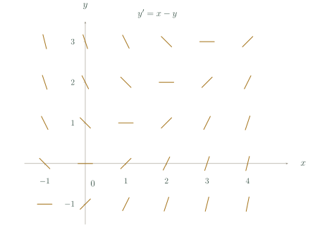
Thirty short equal-length slope segments at x=-1,0,1,2,3,4 and y=-1,0,1,2,3 show y prime=x-y on equal physical coordinate scales. Segments on y=x are horizontal, slopes above that line are negative, and slopes below it are positive.

Follow the directions, not the grid lines

A solution curve must be tangent to the segments it meets. Begin at the given initial point and follow the local directions smoothly as the independent variable increases. For an autonomous equation $y^{'} = f (y)$ , slopes depend only on height, so horizontal rows share a slope.

An equilibrium is a constant solution, not merely a place with zero slope. For an autonomous equation, solve $f (y) = 0$ and inspect signs just above and below: motion toward the equilibrium indicates stability; motion away indicates instability.

02 / WORKED EXAMPLES

See the method in action.

EXAMPLE 01

Worked example

For $y^{'} = x - y$ , find the slopes at $(0, 1)$ , $(1, 1)$ and $(2, 1)$ .

Worked solution

1
Evaluate the slope at the first point.
$y^{'} (0, 1) = 0 - 1 = - 1$
Substitute the coordinates into x minus y; the segment slopes downward as x increases.
2
Evaluate the second and third slopes.
$\begin{array}{c} y^{'} (1, 1) = 1 - 1 = 0 \\ y^{'} (2, 1) = 2 - 1 = 1 \end{array}$
The same height can have different slopes because this equation also depends on x.
3
Describe the three segments.
$- 1, 0, 1$
Draw a descending segment at (0,1), a horizontal segment at (1,1), and an ascending segment at (2,1).

Answer

$- 1, 0, 1$

EXAMPLE 02

Worked example

For $y^{'} = 2 - y$ , describe the equilibrium and nearby solution behaviour.

Worked solution

1
Find and verify the constant solution.
$2 - y = 0 \Rightarrow y = 2, y^{'} = 0 = 2 - 2$
The horizontal function y equals 2 satisfies the equation throughout its domain.
2
Check slopes below and above it.
$\begin{aligned} y < 2 & \Rightarrow y^{'} = 2 - y > 0 \\ y > 2 & \Rightarrow y^{'} = 2 - y < 0 \end{aligned}$
Solutions rise from below and fall from above as x increases.
3
Classify the equilibrium.
$y = 2 is stable$
Both nearby sign regions direct solutions toward the equilibrium height.

Answer

$y = 2$ is a stable equilibrium.

03 / YOUR TURN

Try it yourself.

Check your understanding

For $y^{'} = y - 3$ , is $y = 3$ stable?

Show answer & reasoning

No; it is unstable.

For $y^{'} = y - 3$ , slopes are negative below 3 and positive above 3. Nearby solutions therefore move away from the constant solution $y = 3$ as $x$ increases, so it is unstable.

Keep practising

6 worksheet questions · 12 marks

Open worksheet Worked solutions

Read the questions online

Find slopes for $y^{'} = x y$ at $(1, 2)$ , $(2, - 1)$ and $(0, 3)$ .
2 marks
Where are the slopes zero for $y^{'} = x + y$ ?
2 marks
For $y^{'} = y (4 - y)$ , identify constant equilibria.
2 marks
For $y^{'} = y (4 - y)$ , state slope signs in $y < 0$ , $0 < y < 4$ and $y > 4$ .
2 marks
For $y^{'} = x^{2}$ , what do segments at $(2, 1)$ and $(2, 5)$ have in common?
2 marks
For $y^{'} = - 2 y$ , describe whether a positive solution increases or decreases and whether it crosses the equilibrium.
2 marks

Read the worked solutions

Equivalent correct methods earn the corresponding marks. Include units where asked.

Find slopes for $y^{'} = x y$ at $(1, 2)$ , $(2, - 1)$ and $(0, 3)$ .
2 marks
Multiply the coordinates in each ordered pair.
Use each result as the local line gradient.
$2, - 2, 0$
Where are the slopes zero for $y^{'} = x + y$ ?
2 marks
Set $x + y = 0$ .
Solve for the line $y = - x$ ; this is not a constant equilibrium.
On $y = - x$ .
For $y^{'} = y (4 - y)$ , identify constant equilibria.
2 marks
Constant solutions need derivative zero.
$y (4 - y) = 0$ gives the two values.
$y = 0$ and $y = 4$ .
For $y^{'} = y (4 - y)$ , state slope signs in $y < 0$ , $0 < y < 4$ and $y > 4$ .
2 marks
Check the signs of both factors in each interval.
The sign pattern makes $y = 4$ stable for nearby positive values.
Negative, positive, negative.
For $y^{'} = x^{2}$ , what do segments at $(2, 1)$ and $(2, 5)$ have in common?
2 marks
The equation depends only on $x$ .
At $x = 2$ , $x^{2} = 4$ regardless of $y$ .
Both have gradient $4$ .
For $y^{'} = - 2 y$ , describe whether a positive solution increases or decreases and whether it crosses the equilibrium.
2 marks
For $y > 0$ , $- 2 y < 0$ .
$y = C e^{- 2 x}$ with $C > 0$ stays positive for every finite $x$ .
It decreases toward zero; the nonzero exponential solution does not cross zero.

Checking saved progress…

Curriculum reference & lesson scope

SACE Board of South Australia

Stage 2 Specialist Mathematics topic 6.1–6.2, with the approved school-level rates, differential-equation and motion applications.

Official curriculum source ↗

In this lesson

Understand the idea.

Each short segment is local information

Follow the directions, not the grid lines

See the method in action.

Worked example

Evaluate the slope at the first point.

Evaluate the second and third slopes.

Describe the three segments.

Worked example

Find and verify the constant solution.

Check slopes below and above it.

Classify the equilibrium.

Try it yourself.

Check your understanding

Keep practising