First-derivative graph analysis | Year 11

01 / LEARN

Understand the idea.

Build the sketch from features

Build the graph from exact features: domain, intercepts, stationary points and end behaviour. Solve $f (x) = 0$ for horizontal-axis intercepts, but solve $f^{'} (x) = 0$ for stationary inputs. Substitute the latter into the original function to obtain their heights.

Use derivative signs to connect the known points with the correct rising and falling sections. The leading term determines polynomial end behaviour. Repeated roots need care: an even-multiplicity root touches the axis, while an odd-multiplicity root crosses it.

The graph of y equals x cubed minus three x, shown from x minus two to two and y minus three to three. Turning points are visible without coordinate annotations.

Check what is determined

A derivative describes slope behaviour but does not locate the graph vertically. Adding a constant shifts the whole graph without changing its derivative. A supplied point can distinguish between these vertically shifted curves and fix the missing height information.

A graphing tool can help check the assembled shape, but exact intercepts and classifications come from the equations. If the screen suggests an extra turn, revisit the derivative and viewing window. A sketch should label key coordinates and show consistent end behaviour.

02 / WORKED EXAMPLES

See the method in action.

EXAMPLE 01

Worked example 1

Analyse $f (x) = x^{3} - 3 x^{2}$ .

The graph of y equals x cubed minus three x squared, shown from x minus one to four and y minus six to six. Original gold annotations identify local maximum zero, zero, local minimum two, minus four, and crossing three, zero.

Worked solution

1
Factor the function and identify intercepts.
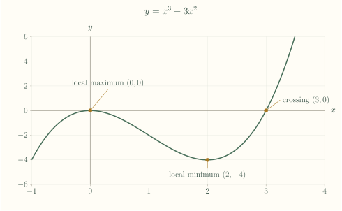
$\begin{aligned} f (x) & = x^{2} (x - 3) \\ f (x) = 0 & ⟹ x = 0 or x = 3 \end{aligned}$
The intercepts are $(0, 0)$ and $(3, 0)$ ; the double root at zero indicates contact without crossing.
2
Find the stationary inputs.
$\begin{aligned} f^{'} (x) & = 3 x^{2} - 6 x = 3 x (x - 2) \\ f^{'} (x) = 0 & ⟹ x = 0 or x = 2 \end{aligned}$
The tangent is horizontal at the roots of the derivative.
3
Calculate the stationary coordinates.
$\begin{aligned} f (0) & = 0 \\ f (2) & = 8 - 12 = - 4 \end{aligned}$
The original function gives $(0, 0)$ and $(2, - 4)$ .
4
Classify using derivative signs.
$\begin{aligned} x < 0 : & f^{'} (x) > 0 \\ 0 < x < 2 : & f^{'} (x) < 0 \\ x > 2 : & f^{'} (x) > 0 \end{aligned}$
The factored derivative shows a local maximum at $(0, 0)$ and a local minimum at $(2, - 4)$ .
5
Complete the cubic’s overall shape.
$\begin{aligned} x \to - \infty : & f (x) \to - \infty \\ x \to \infty : & f (x) \to \infty \end{aligned}$
The positive cubic term determines both ends: the graph rises to touch at zero, dips to the minimum, then rises through $(3, 0)$ .

Answer

A cubic touching the axis at its local maximum (0,0), dipping to (2,−4), then crossing at (3,0).

EXAMPLE 02

Worked example 2

Analyse $g (x) = - x^{3} + 3 x$ .

The graph of y equals minus x cubed plus three x, from x minus two to two and y minus three to three. Original annotations mark local minimum minus one, minus two and local maximum one, two.

Worked solution

1
Find all axis intercepts.
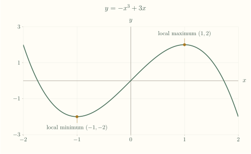
$\begin{aligned} g (x) & = x (3 - x^{2}) \\ g (x) = 0 & ⟹ x = - \sqrt{3}, 0, \sqrt{3} \end{aligned}$
All three roots are simple, so the curve crosses the horizontal axis at each; the vertical-axis intercept is $(0, 0)$ .
2
Find the stationary inputs.
$\begin{aligned} g^{'} (x) & = 3 - 3 x^{2} = 3 (1 - x) (1 + x) \\ g^{'} (x) = 0 & ⟹ x = - 1 or x = 1 \end{aligned}$
These are the only zeros of the derivative.
3
Calculate the stationary heights.
$\begin{aligned} g (- 1) & = - {(- 1)}^{3} + 3 (- 1) = - 2 \\ g (1) & = - 1 + 3 = 2 \end{aligned}$
The original cubic gives the stationary coordinates $(- 1, - 2)$ and $(1, 2)$ .
4
Determine the rising and falling intervals.
$\begin{aligned} x < - 1 : & g^{'} (x) < 0 \\ - 1 < x < 1 : & g^{'} (x) > 0 \\ x > 1 : & g^{'} (x) < 0 \end{aligned}$
The derivative is positive between its roots and negative outside, giving a local minimum $(- 1, - 2)$ and local maximum $(1, 2)$ .
5
Check the ends before sketching.
$\begin{aligned} x \to - \infty : & g (x) \to \infty \\ x \to \infty : & g (x) \to - \infty \end{aligned}$
The negative leading cubic term places the left end high and the right end low, consistent with decreasing outer sections.

Answer

A negative-leading cubic increasing on (−1,1), decreasing outside.

03 / YOUR TURN

Try it yourself.

Check your understanding

f and g have the same derivative and g(0)=f(0)+4. How are their graphs related?

Show answer & reasoning

g is shifted vertically upwards by 4.

On their common interval, equal derivatives mean the difference $g - f$ is constant. Since $g (0) - f (0) = 4$ , this constant is 4: $g (x) = f (x) + 4$ , a vertical shift upwards by 4.

Keep practising

6 worksheet questions · 24 marks

Open worksheet Worked solutions

Read the questions online

List intercepts, stationary point and monotonic intervals of $f (x) = x^{2} - 4 x + 3$ .
5 marks
Analyse $f (x) = x^{3} - 3 x^{2}$ .
5 marks
A differentiable function has derivative zero at $x = - 2$ and $x = 1$ . Its derivative is positive for $x < - 2$ , negative for $- 2 < x < 1$ , and positive for $x > 1$ . State the stationary types.
3 marks
Find roots and stationary points of $g (x) = x^{3} - 3 x$ .
5 marks
A straight-line function has $f^{'} (x) = 2$ and $f (0) = - 3$ . Find $f$ .
3 marks
Why can the derivative alone not determine vertical position?
3 marks

Read the worked solutions

Equivalent correct methods earn the corresponding marks. Include units where asked.

List intercepts, stationary point and monotonic intervals of $f (x) = x^{2} - 4 x + 3$ .
5 marks
$f = (x - 1) (x - 3)$ ; $f^{'} = 2 x - 4$ .
Evaluate $f$ at 0 and 2 and use derivative signs.
Roots 1,3; y-intercept 3; minimum $(2, - 1)$ ; decreasing $x < 2$ , increasing $x > 2$ .
Analyse $f (x) = x^{3} - 3 x^{2}$ .
5 marks
$f = x^{2} (x - 3)$ and $f^{'} = 3 x (x - 2)$ .
The derivative signs are +, −, +.
Intercepts $(0, 0), (3, 0)$ ; maximum $(0, 0)$ ; minimum $(2, - 4)$ .
A differentiable function has derivative zero at $x = - 2$ and $x = 1$ . Its derivative is positive for $x < - 2$ , negative for $- 2 < x < 1$ , and positive for $x > 1$ . State the stationary types.
3 marks
The signs change + to − at $- 2$ and − to + at 1.
No heights can be found from this information alone.
Maximum at $x = - 2$ ; minimum at $x = 1$ .
Find roots and stationary points of $g (x) = x^{3} - 3 x$ .
5 marks
$g = x (x^{2} - 3)$ and $g^{'} = 3 (x - 1) (x + 1)$ .
Use signs +, −, + and evaluate $g$ at $\pm 1$ .
Roots $0, \pm \sqrt{3}$ ; maximum $(- 1, 2)$ , minimum $(1, - 2)$ .
A straight-line function has $f^{'} (x) = 2$ and $f (0) = - 3$ . Find $f$ .
3 marks
A line of gradient 2 has form $2 x + c$ .
The intercept condition makes $c = - 3$ .
$f (x) = 2 x - 3$
Why can the derivative alone not determine vertical position?
3 marks
For example $x^{2}$ and $x^{2} + 5$ both have derivative $2 x$ but different heights.
Adding a constant leaves the derivative unchanged.

Checking saved progress…

Curriculum reference & lesson scope

SACE Board of South Australia

Stage 1 Mathematics topic 6: rates of change, derivatives and applications. Introductory polynomial calculus with explicit modelling and interpretation.

Official curriculum source ↗

In this lesson

Understand the idea.

Build the sketch from features

Check what is determined

See the method in action.

Worked example 1

Factor the function and identify intercepts.

Find the stationary inputs.

Calculate the stationary coordinates.

Classify using derivative signs.

Complete the cubic’s overall shape.

Worked example 2

Find all axis intercepts.

Find the stationary inputs.

Calculate the stationary heights.

Determine the rising and falling intervals.

Check the ends before sketching.

Try it yourself.

Check your understanding

Keep practising