Normal-curve features and the 68–95–99.7 rule | Year 11

01 / LEARN

Understand the idea.

Area under the curve represents a proportion

A normal model is a continuous, symmetric, bell-shaped distribution. Its mean $μ$ fixes the centre and its standard deviation $σ > 0$ fixes the horizontal scale. The ideal model has equal mean, median and mode.

Total area under the curve is $1$ . An interval probability is the area above that interval, rather than the curve's height. A single exact value has zero probability in this continuous model, although any interval around it can have positive probability.

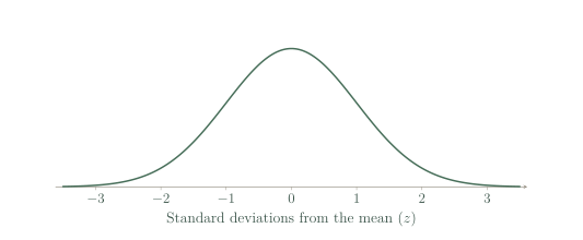
A smooth standard-normal density is centred at z zero and drawn from minus 3.5 to 3.5. The horizontal axis is labelled minus three to three standard deviations from the mean; no numerical density or probability height is marked.

Use the empirical rule as an approximation

The 68–95–99.7 rule estimates the proportions within one, two and three standard deviations of a normal mean. These are central intervals extending equally to both sides; symmetry splits each remaining outside proportion equally between the tails.

These percentages are rounded approximations, useful when an estimate is requested. Use normal-distribution technology for more accurate probabilities, and check that a bell-shaped normal model is reasonable before applying the rule to measured data, especially if the data are strongly skewed.

\begin{aligned} μ \pm σ & : 68 % \\ μ \pm 2 σ & : 95 % \\ μ \pm 3 σ & : 99.7 % \end{aligned}

02 / WORKED EXAMPLES

See the method in action.

EXAMPLE 01

A central interval

A normal model has mean 70 and standard deviation 8. Estimate the proportion between 54 and 86.

Worked solution

1
Measure each endpoint from the mean.
$\begin{aligned} \frac{54 - 70}{8} & = - 2 \\ \frac{86 - 70}{8} & = 2 \end{aligned}$
Dividing each difference by 8 expresses the endpoint in standard deviations.
2
Identify the central normal interval.
$54 = μ - 2 σ, 86 = μ + 2 σ$
The interval extends exactly two standard deviations either side of the mean.
3
Apply the empirical rule.
$P (54 < X < 86) \approx 0.95$
About 95% of a normal model lies within two standard deviations, so the estimated proportion is 95%.

Answer

About 95%.

EXAMPLE 02

An upper tail

Bottle-fill volumes are approximately normal with mean 500 mL and standard deviation 4 mL. Estimate how many of 2,000 bottles exceed 508 mL.

Worked solution

1
Locate the upper cutoff.
$\frac{508 - 500}{4} = 2$
The 508 mL cutoff is two standard deviations above the mean.
2
Find the approximate upper-tail proportion.
$P (X > 508) \approx \frac{1 - 0.95}{2} = 0.025$
The central 95% leaves about 5% outside, split equally between the two tails.
3
Convert the proportion into an expected count.
$2000 \times 0.025 = 50$
The empirical-rule estimate is about 50 bottles; the actual count in a batch can vary.

Answer

About 50 bottles.

03 / YOUR TURN

Try it yourself.

Check your understanding

Estimate the proportion below the mean in a normal model.

Show answer & reasoning

50%.

A normal curve is symmetric about its mean and has no probability concentrated at one point. Half its area lies below the mean, giving $50 %$ .

Keep practising

6 worksheet questions · 13 marks

Open worksheet Worked solutions

Read the questions online

A normal model has mean 30 and sd 5. Give the interval containing about 68%.
2 marks
For the same model, estimate the proportion above 40.
2 marks
Estimate the proportion between the mean and 1 standard deviation above it.
2 marks
Estimate the proportion more than 3 standard deviations from the mean.
2 marks
A normal model has mean 100 and sd 15. Estimate how many of 800 observations lie from 85 to 115.
2 marks
A distribution of waiting times has a long right tail. Is it justified to assume 68% lie within one sd? Explain.
3 marks

Read the worked solutions

Equivalent correct methods earn the corresponding marks. Include units where asked.

A normal model has mean 30 and sd 5. Give the interval containing about 68%.
2 marks
Use mean $\pm 1$ standard deviation.
25 to 35.
For the same model, estimate the proportion above 40.
2 marks
40 is 2 standard deviations above 30; split the 5% outside $\pm 2$ standard deviations into two tails.
About 2.5%.
Estimate the proportion between the mean and 1 standard deviation above it.
2 marks
Take half of the central 68%.
About 34%.
Estimate the proportion more than 3 standard deviations from the mean.
2 marks
$100 % - 99.7 % = 0.3 %$ , including both tails.
About 0.3%.
A normal model has mean 100 and sd 15. Estimate how many of 800 observations lie from 85 to 115.
2 marks
The interval is $\pm 1$ standard deviation, so $0.68 \times 800 = 544$ .
About 544.
A distribution of waiting times has a long right tail. Is it justified to assume 68% lie within one sd? Explain.
3 marks
The empirical rule is specific to an approximately normal shape.
A long right tail gives reason to question that model.
No, not from that information.

Checking saved progress…

Curriculum reference & lesson scope

SACE Board of South Australia

Stage 1 Mathematics: counting, binomial expansion, data, samples, summary measures and introductory normal distributions. These lessons provide the Counting and Statistics strand of the approved Methods preparation route.

Official curriculum source ↗

In this lesson

Understand the idea.

Area under the curve represents a proportion

Use the empirical rule as an approximation

See the method in action.

A central interval

Measure each endpoint from the mean.

Identify the central normal interval.

Apply the empirical rule.

An upper tail

Locate the upper cutoff.

Find the approximate upper-tail proportion.

Convert the proportion into an expected count.

Try it yourself.

Check your understanding

Keep practising