Sample means and the central-limit idea | Year 12

01 / LEARN

Understand the idea.

A mean varies between samples

Imagine repeatedly taking independent samples of one fixed size and calculating a mean each time. These means form a sampling distribution. Its centre is $E (\bar{X}) = μ$ , while its variance is $Var (\bar{X}) = \frac{σ^{2}}{n}$ : averaging preserves the centre and reduces variability.

The standard deviation of those means is the standard error, $\frac{σ}{\sqrt{n}}$ . Keep it separate from $σ$ , the spread of individual observations. A probability about an average therefore uses the mean distribution, not the individual-observation distribution.

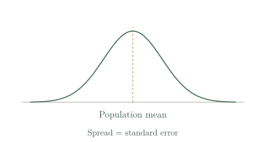
\begin{aligned} E (\bar{X}) & = μ \\ SD (\bar{X}) & = \frac{σ}{\sqrt{n}} \end{aligned}

A smooth symmetric bell-shaped sampling distribution is centred at the dashed line labelled Population mean. Its spread is labelled standard error. The curve is schematic: no numerical population mean, sample size or standard error is specified.

When a bell-shaped model is justified

If independent observations come from a normal population, their sample mean is exactly normal at every sample size. For independent, identically distributed observations with finite variance, the central limit theorem instead supports an increasingly accurate normal approximation as sample size grows.

There is no sample size that guarantees accuracy for every population. Strong skewness or heavy tails can require more averaging. Check independence separately: adjacent readings from a drifting sensor may share an influence, so their effective information need not match the reading count.

02 / WORKED EXAMPLES

See the method in action.

EXAMPLE 01

Exact sampling model

Fill volumes are normal with mean 500 mL and standard deviation 12 mL. Model the mean of 36 independent fills.

Worked solution

1
Keep the population mean as the centre.
$E (\bar{X}) = μ = 500 mL$
The mean of independent observations from this population is an unbiased estimator of its mean.
2
Calculate the standard error.
$SD (\bar{X}) = \frac{12}{\sqrt{36}} = 2 mL$
The spread of averages is the individual spread divided by the square root of sample size.
3
Write the distribution with its variance.
$\bar{X} \sim N (500, 2^{2})$
The population is normal and the fills are independent, so this normal model is exact; the second parameter is variance.

Answer

$\bar{X} \sim N (500, 2^{2})$ .

EXAMPLE 02

Probability for an average

For that sample mean, find $P (498 < \bar{X} < 502)$ .

Worked solution

1
Use the sample-mean standard deviation.
$Z = \frac{\bar{X} - 500}{2} \sim N (0, 1)$
These bounds concern the average of 36 fills, whose standard deviation is 2 mL.
2
Standardise both endpoints.
$\begin{aligned} \frac{498 - 500}{2} & = - 1 \\ \frac{502 - 500}{2} & = 1 \end{aligned}$
Subtracting the mean and dividing by the positive standard error preserves the order of the bounds.
3
Evaluate the central normal probability.
$\begin{aligned} P (498 < \bar{X} < 502) & = Φ (1) - Φ (- 1) \\ \approx 0.6827 \end{aligned}$
The required area is the upper cumulative probability minus the lower cumulative probability.

Answer

Approximately 0.6827.

03 / YOUR TURN

Try it yourself.

Check your understanding

For population mean 40, standard deviation 15 and n = 25, find the sample-mean centre and standard deviation.

Show answer & reasoning

40 and 3.

The centre remains $E (\bar{X}) = 40$ . Its standard deviation is $\frac{15}{\sqrt{25}} = 3$ , using the independent-observation model. These two quantities alone do not establish that the distribution is normal.

Keep practising

6 worksheet questions · 12 marks

Open worksheet Worked solutions

Read the questions online

For $μ = 72, σ = 18, n = 36$ , find the mean and variance of $\bar{X}$ .
2 marks
Normal observations have mean 100 and standard deviation 20. Model a mean of 16 independent observations.
2 marks
For the previous model, find $P (\bar{X} > 110)$ .
2 marks
Why need a mean of four highly right-skewed observations not be approximately normal?
2 marks
What changes as independent sample size grows for a non-normal finite-variance population?
2 marks
Why can 100 consecutive readings from one drifting sensor fail independence?
2 marks

Read the worked solutions

Equivalent correct methods earn the corresponding marks. Include units where asked.

For $μ = 72, σ = 18, n = 36$ , find the mean and variance of $\bar{X}$ .
2 marks
$E (\bar{X}) = 72$ ; $Var (\bar{X}) = \frac{18^{2}}{36} = 9$ .
72 and 9.
Normal observations have mean 100 and standard deviation 20. Model a mean of 16 independent observations.
2 marks
The standard error is $\frac{20}{\sqrt{16}} = 5$ .
$\bar{X} \sim N (100, 5^{2})$ .
For the previous model, find $P (\bar{X} > 110)$ .
2 marks
$z = \frac{110 - 100}{5} = 2$ .
$1 - Φ (2) = 0.022750 \dots$ .
Approximately 0.0228.
Why need a mean of four highly right-skewed observations not be approximately normal?
2 marks
The central limit theorem is a limiting result, not a guarantee for every small sample.
A sample of four may be too small to average away strong skewness.
What changes as independent sample size grows for a non-normal finite-variance population?
2 marks
Its standard deviation is $\frac{σ}{\sqrt{n}}$ ; its expectation is $μ$ .
The mean distribution tends towards normality and becomes narrower; its centre remains the population mean.
Why can 100 consecutive readings from one drifting sensor fail independence?
2 marks
A large reading count is not evidence that the observations are independent.
Adjacent readings can share drift and be correlated.

Checking saved progress…

Curriculum reference & lesson scope

SACE Board of South Australia

Stage 2 Mathematical Methods: sampling distributions and confidence intervals for means and proportions. Mean tasks distinguish known population spread from sufficiently large-sample estimated-spread normal intervals. Repeated-interval computational simulation, approximation conditions, design and interpretation are included.

Official curriculum source ↗

In this lesson

Understand the idea.

A mean varies between samples

When a bell-shaped model is justified

See the method in action.

Exact sampling model

Keep the population mean as the centre.

Calculate the standard error.

Write the distribution with its variance.

Probability for an average

Use the sample-mean standard deviation.

Standardise both endpoints.

Evaluate the central normal probability.

Try it yourself.

Check your understanding

Keep practising