Stationary-point classification | Year 12

01 / LEARN

Understand the idea.

Find then classify

A stationary point is a point on the curve with $f^{'} (x) = 0$ . Solve this equation within the original domain, then calculate each height from $f (x)$ before classifying the point.

Read the first derivative on both sides: positive to negative gives a local maximum, and negative to positive gives a local minimum. If it keeps the same sign, the function keeps moving in the same direction.

A useful short test

At a stationary input $a$ , the second-derivative test is a shortcut: $f^{''} (a) > 0$ gives a local minimum and $f^{''} (a) < 0$ gives a local maximum. These conclusions require a stationary input.

If $f^{''} (a) = 0$ , the test gives no classification. Use a first-derivative sign argument instead. Both $x^{3}$ and $x^{4}$ have zero first and second derivatives at zero, yet only one has a minimum there.

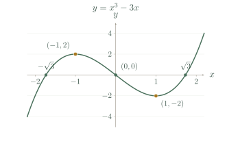
Labelled graph of y=x cubed minus 3x, showing roots negative square root 3, zero and square root 3, maximum (-1,2), minimum (1,-2), with numbered axes.

02 / WORKED EXAMPLES

See the method in action.

EXAMPLE 01

Two stationary points

Classify the stationary points of $f (x) = x^{3} - 3 x$ .

Worked solution

1
Find all stationary inputs.
$\begin{aligned} f^{'} (x) & = 3 x^{2} - 3 = 3 (x - 1) (x + 1) \\ f^{'} (x) = 0 & ⟹ x = - 1 or x = 1 \end{aligned}$
A product is zero only when at least one factor is zero.
2
Classify using the second derivative.
$\begin{aligned} f^{''} (x) & = 6 x \\ f^{''} (- 1) & = - 6 < 0 \\ f^{''} (1) & = 6 > 0 \end{aligned}$
A negative second derivative at a stationary point gives a maximum; a positive one gives a minimum.
3
Calculate the heights.
$f (- 1) = - 1 + 3 = 2, f (1) = 1 - 3 = - 2$
The original function supplies each y-coordinate.
4
State the classifications as points.
$Local maximum (- 1, 2); local minimum (1, - 2)$
Each classification is attached to its corresponding input and height.

Answer

Local maximum $(- 1, 2)$ ; local minimum $(1, - 2)$ .

EXAMPLE 02

When the second-derivative test is inconclusive

Classify the stationary point of $y = x^{4}$ .

Worked solution

1
Find the stationary point.
$y^{'} = 4 x^{3} = 0 x = 0, y (0) = 0$
Zero is the only input with a horizontal tangent.
2
Check the shortcut test.
$y^{''} = 12 x^{2}, y^{''} (0) = 0$
A zero value makes the second-derivative test inconclusive.
3
Determine the first-derivative signs.
$x < 0 ⟹ 4 x^{3} < 0, x > 0 ⟹ 4 x^{3} > 0$
Cubing preserves the sign of x.
4
Conclude the classification.
$Local minimum at (0, 0)$
The curve decreases into the point and increases away from it.

Answer

Local minimum $(0, 0)$ .

03 / YOUR TURN

Try it yourself.

Check your understanding

What does a change of $f^{'}$ from positive to negative show?

Show answer & reasoning

A local maximum.

A positive first derivative before a stationary point means the curve rises towards it. A negative derivative afterwards means it falls away, so this change indicates a local maximum.

Keep practising

6 worksheet questions · 15 marks

Open worksheet Worked solutions

Read the questions online

Find and classify the stationary point of $y = x^{2} - 6 x + 5$ .
2 marks
Find and classify the stationary point of $y = - x^{2} + 4 x$ .
2 marks
Classify the stationary points of $y = x^{3} - 3 x^{2}$ .
3 marks
Explain why the stationary point of $y = x^{3}$ is not an extremum.
2 marks
Classify the stationary point of $y = x e^{- x}$ .
3 marks
Can a local maximum fail to be an absolute maximum on an unbounded domain? Give an example.
3 marks

Read the worked solutions

Equivalent correct methods earn the corresponding marks. Include units where asked.

Find and classify the stationary point of $y = x^{2} - 6 x + 5$ .
2 marks
The derivative is $2 x - 6$ , zero at 3.
The second derivative is 2; the height is $- 4$ .
Local minimum $(3, - 4)$ .
Find and classify the stationary point of $y = - x^{2} + 4 x$ .
2 marks
The derivative is $- 2 x + 4$ , zero at 2.
The second derivative is $- 2$ .
Local maximum $(2, 4)$ .
Classify the stationary points of $y = x^{3} - 3 x^{2}$ .
3 marks
The derivative is $3 x (x - 2)$ .
The second derivative $6 x - 6$ is negative at 0 and positive at 2.
Local maximum $(0, 0)$ ; local minimum $(2, - 4)$ .
Explain why the stationary point of $y = x^{3}$ is not an extremum.
2 marks
The derivative is $3 x^{2}$ .
There is no increasing/decreasing reversal.
The derivative is positive on both sides of zero.
Classify the stationary point of $y = x e^{- x}$ .
3 marks
The derivative is $e^{- x} (1 - x)$ .
Its sign changes from positive to negative at 1.
Local maximum $(1, e^{- 1})$ .
Can a local maximum fail to be an absolute maximum on an unbounded domain? Give an example.
3 marks
A local maximum compares nearby inputs only.
As $x$ grows, $x^{3} - 3 x$ grows without bound.
Yes: $x^{3} - 3 x$ has a local maximum at $(- 1, 2)$ but is unbounded above.

Checking saved progress…

Curriculum reference & lesson scope

SACE Stage 2 Mathematical Methods

Further differentiation and applications from the current SACE Methods outline. Logarithmic derivatives have their own chapter; integration follows later. Trigonometric calculus uses radians.

Official curriculum source ↗

In this lesson

Understand the idea.

Find then classify

A useful short test

See the method in action.

Two stationary points

Find all stationary inputs.

Classify using the second derivative.

Calculate the heights.

State the classifications as points.

When the second-derivative test is inconclusive

Find the stationary point.

Check the shortcut test.

Determine the first-derivative signs.

Conclude the classification.

Try it yourself.

Check your understanding

Keep practising