Curve analysis | Year 12 | Ascent Library

01 / LEARN

Understand the idea.

Build a complete picture

A convincing curve sketch combines domain, intercepts and end behaviour with derivative information. Find where $f^{'}$ is positive, negative or zero, then use $f^{''}$ to locate changes in concavity. Every labelled feature should agree.

A calculator graph can check the overall picture, but its window may hide a root, asymptote or turning point. Algebra and derivative signs explain why the features occur and which intervals they describe.

Respect disconnected domains

For a disconnected domain, include excluded inputs when dividing sign intervals. A vertical asymptote separates branches even when neither branch contains a stationary point near that boundary. Never join across an input missing from the domain.

Label intercepts, stationary points and asymptotes with a useful scale. To identify a slant asymptote $y = m x + c$ , check that the difference between the function and that line tends to zero as $x$ tends towards infinity or negative infinity.

Labelled graph of y=x cubed minus 3x, showing roots negative square root 3, zero and square root 3, maximum (-1,2), minimum (1,-2), with numbered axes.

02 / WORKED EXAMPLES

See the method in action.

EXAMPLE 01

A cubic sketch from its features

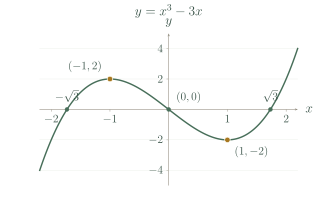
Describe a sketch of $y = x^{3} - 3 x$ .

Worked solution

1
Find the roots and symmetry.
$\begin{aligned} y & = x (x^{2} - 3) = 0 x = - \sqrt{3}, 0, \sqrt{3} \\ f (- x) & = - f (x) \end{aligned}$
The factorisation gives the intercepts, and odd symmetry relates opposite points.
2
Find stationary points and monotonic intervals.
$\begin{aligned} f^{'} (x) & = 3 (x - 1) (x + 1) \\ f^{'} > 0 & on (- \infty, - 1) and (1, \infty) \\ f^{'} < 0 & on (- 1, 1) \end{aligned}$
The two derivative factors have the same sign outside the roots and opposite signs between them.
3
Label the turning points.
$f (- 1) = 2, f (1) = - 2$
The derivative changes positive to negative at (-1,2), then negative to positive at (1,-2).
4
Find concavity and the inflection.
$f^{''} (x) = 6 x, inflection (0, 0)$
Concavity changes from down for x<0 to up for x>0.
5
Complete the end behaviour.
$x \to - \infty ⟹ y \to - \infty, x \to \infty ⟹ y \to \infty$
The positive cubic leading term dominates at large input magnitudes.

Answer

An odd cubic with the three labelled roots and two stationary points.

EXAMPLE 02

Separate branches of a rational curve

Find the key features of $y = x + 1 / x$ .

Worked solution

1
Record the domain, intercepts and asymptotes.
$\begin{aligned} x & \neq 0, x + \frac{1}{x} = 0 ⟹ x^{2} + 1 = 0 \\ f (x) - x & = \frac{1}{x} \to 0 (x \to \pm \infty) \end{aligned}$
There are no real x-intercepts or y-intercept; the asymptotes are x=0 and y=x.
2
Solve the stationary equation.
$f^{'} (x) = 1 - \frac{1}{x^{2}} = \frac{(x - 1) (x + 1)}{x^{2}} = 0 x = \pm 1$
The denominator is positive throughout the domain, so it contributes no sign change.
3
Use derivative signs to classify the points.
$\begin{aligned} f^{'} > 0 & for x < - 1 and x > 1 \\ f^{'} < 0 & for - 1 < x < 0 and 0 < x < 1 \\ f (- 1) & = - 2, f (1) = 2 \end{aligned}$
The changes give a local maximum (-1,-2) and a local minimum (1,2).
4
Describe the two separate branches.
$\begin{aligned} x \to 0^{-} & ⟹ f (x) \to - \infty \\ x \to 0^{+} & ⟹ f (x) \to \infty \end{aligned}$
The reciprocal term dominates near zero; neither branch passes through the excluded input.
5
Check the bend on each branch.
$f^{''} (x) = \frac{2}{x^{3}} < 0 (x < 0), f^{''} (x) > 0 (x > 0)$
The negative branch is concave down and the positive branch concave up; zero itself is not an inflection point.

Answer

Two branches, with no real x-intercepts and the stated asymptotes.

03 / YOUR TURN

Try it yourself.

Check your understanding

How many real x-intercepts has $y = x^{2} + 1$ ?

Show answer & reasoning

None.

Since $x^{2} \geq 0$ for every real $x$ , $x^{2} + 1 \geq 1 > 0$ . It can never equal zero, so the graph has no real x-intercepts.

Keep practising

6 worksheet questions · 17 marks

Open worksheet Worked solutions

Read the questions online

Find all intercepts of $y = x^{3} - 4 x$ .
2 marks
State increasing intervals for $y = x^{3} - 3 x$ .
2 marks
For $y = x^{4} - 2 x^{2}$ , find all stationary coordinates.
3 marks
Find the vertical and oblique asymptotes of $y = x + \frac{1}{x}$ .
2 marks
Sketch $y = e^{- x}$ by stating its intercept, monotonicity, concavity and asymptote.
4 marks
For $f (x) = x^{3} - 3 x$ on $[- 2, 2]$ , find the absolute maximum and minimum.
4 marks

Read the worked solutions

Equivalent correct methods earn the corresponding marks. Include units where asked.

Find all intercepts of $y = x^{3} - 4 x$ .
2 marks
Factor as $x (x - 2) (x + 2)$ .
Set each factor to zero.
x-intercepts $(- 2, 0), (0, 0), (2, 0)$ ; y-intercept $(0, 0)$ .
State increasing intervals for $y = x^{3} - 3 x$ .
2 marks
The derivative is $3 (x^{2} - 1)$ .
It is positive when $∣ x ∣ > 1$ .
$(- \infty, - 1)$ and $(1, \infty)$ .
For $y = x^{4} - 2 x^{2}$ , find all stationary coordinates.
3 marks
The derivative is $4 x (x^{2} - 1)$ .
Evaluate the original function at $- 1, 0, 1$ .
$(- 1, - 1), (0, 0), (1, - 1)$ .
Find the vertical and oblique asymptotes of $y = x + \frac{1}{x}$ .
2 marks
The reciprocal term is undefined at zero.
It tends to zero as $∣ x ∣$ becomes large.
$x = 0$ and $y = x$ .
Sketch $y = e^{- x}$ by stating its intercept, monotonicity, concavity and asymptote.
4 marks
The first derivative is negative and the second positive.
The exponential remains positive and tends to zero as $x$ increases.
Intercept $(0, 1)$ ; decreasing; concave up; horizontal asymptote $y = 0$ .
For $f (x) = x^{3} - 3 x$ on $[- 2, 2]$ , find the absolute maximum and minimum.
4 marks
Check stationary inputs $- 1, 1$ and endpoints $- 2, 2$ .
The values are respectively $2, - 2, - 2, 2$ .
Maximum 2 at $x = - 1, 2$ ; minimum $- 2$ at $x = - 2, 1$ .

Checking saved progress…

Curriculum reference & lesson scope

SACE Stage 2 Mathematical Methods

Further differentiation and applications from the current SACE Methods outline. Logarithmic derivatives have their own chapter; integration follows later. Trigonometric calculus uses radians.

Official curriculum source ↗

In this lesson

Understand the idea.

Build a complete picture

Respect disconnected domains

See the method in action.

A cubic sketch from its features

Find the roots and symmetry.

Find stationary points and monotonic intervals.

Label the turning points.

Find concavity and the inflection.

Complete the end behaviour.

Separate branches of a rational curve

Record the domain, intercepts and asymptotes.

Solve the stationary equation.

Use derivative signs to classify the points.

Describe the two separate branches.

Check the bend on each branch.

Try it yourself.

Check your understanding

Keep practising