Normal distributions | Year 12 | Mathematical Methods

01 / LEARN

Understand the idea.

A bell-shaped family

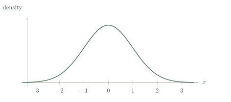
A normal distribution is symmetric and bell-shaped, with mean, median and mode at the same centre. Standard deviation controls spread: increasing it widens and lowers the curve while total area stays $1$ . The theoretical support is all real numbers.

Here $N (μ, σ^{2})$ lists the mean and variance. A calculator may instead request standard deviation $σ$ . Check its input label. For a nonnegative measurement, a substantial predicted negative tail can indicate that a normal model is unsuitable.

A standard normal density is shown from x=-3.5 to 3.5, centred at zero, with horizontal labels from -3 to 3. Density heights remain unnumbered and no tail or probability region is added.

Use symmetry and sensible approximations

Symmetry places half the probability on each side of the mean. The empirical rule estimates about $68 %$ , $95 %$ and $99.7 %$ within one, two and three standard deviations. These are quick checks on a calculated area.

Use a normal cumulative calculation when greater precision is needed, and sketch the intended interval first. Distinguish an individual measurement from a sample mean: independent averaging reduces the spread, so the same bounds can give very different probabilities.

02 / WORKED EXAMPLES

See the method in action.

EXAMPLE 01

Read the parameters

$X \sim N (64, 25)$ . State its mean, standard deviation and P(X>64).

Worked solution

1
Read the mean and variance in the stated convention.
$μ = 64, σ^{2} = 25$
The second parameter is variance in the notation used here.
2
Take the square root of the variance.
$σ = \sqrt{25} = 5$
Standard deviation is the positive scale parameter.
3
Use normal symmetry at the mean.
$P (X > 64) = \frac{1}{2} = 0.5$
Half the continuous distribution lies strictly above its centre.

Answer

64; 5; 0.5.

EXAMPLE 02

Estimate a central region

A normal variable has mean 100 and standard deviation 8. Estimate P(84<X<116).

Worked solution

1
Express both bounds in standard-deviation units.
$84 = 100 - 2 (8), 116 = 100 + 2 (8)$
The requested interval extends two standard deviations on either side of the mean.
2
Apply the empirical rule.
$P (84 < X < 116) \approx 0.95$
About 95% of a normal distribution lies within two standard deviations.
3
Distinguish the estimate from the calculated area.
$P (- 2 < Z < 2) \approx 0.9545$
The more precise normal area is about 95.45%, consistent with the requested estimate of about 95%.

Answer

About 95%.

03 / YOUR TURN

Try it yourself.

Check your understanding

$X \sim N (50, 16)$ . Find its standard deviation and median.

Show answer & reasoning

4 and 50.

The standard deviation is $\sqrt{16} = 4$ . Normal symmetry makes the median equal the mean, so the median is $50$ .

Keep practising

6 worksheet questions · 12 marks

Open worksheet Worked solutions

Read the questions online

$X \sim N (12, 9)$ . State mean and standard deviation.
2 marks
A normal model has mean 40 and standard deviation 6. Give the central two-SD interval.
2 marks
Why is the probability at exactly the normal mean not 0.5?
2 marks
Does doubling the standard deviation change the total density area?
2 marks
A waiting-time distribution has a very long right tail. Is a symmetric normal model automatically suitable?
2 marks
$X \sim N (30, 4)$ . Estimate $P (28 < X < 32)$ using the empirical rule.
2 marks

Read the worked solutions

Equivalent correct methods earn the corresponding marks. Include units where asked.

$X \sim N (12, 9)$ . State mean and standard deviation.
2 marks
The parameters are mean and variance.
12 and 3.
A normal model has mean 40 and standard deviation 6. Give the central two-SD interval.
2 marks
$40 \pm 2 (6)$ .
$[28, 52]$ .
Why is the probability at exactly the normal mean not 0.5?
2 marks
A half-line has probability 0.5; one point has no area.
A singleton has probability zero.
Does doubling the standard deviation change the total density area?
2 marks
The curve widens and lowers.
No; it stays one.
A waiting-time distribution has a very long right tail. Is a symmetric normal model automatically suitable?
2 marks
The shape is inconsistent with a normal model; inspect actual behaviour.
No.
$X \sim N (30, 4)$ . Estimate $P (28 < X < 32)$ using the empirical rule.
2 marks
The endpoints are one standard deviation from the mean.
About 0.68.

Checking saved progress…

Curriculum reference & lesson scope

SACE Board of South Australia

Stage 2 Mathematical Methods: continuous random variables, normal distributions and sampling distributions of sample means. Original lessons and practice.

Official curriculum source ↗

In this lesson

Understand the idea.

A bell-shaped family

Use symmetry and sensible approximations

See the method in action.

Read the parameters

Read the mean and variance in the stated convention.

Take the square root of the variance.

Use normal symmetry at the mean.

Estimate a central region

Express both bounds in standard-deviation units.

Apply the empirical rule.

Distinguish the estimate from the calculated area.

Try it yourself.

Check your understanding

Keep practising