
Understand the idea.
Observed minus predicted
A residual compares one observed response with its prediction at the same predictor value: . Positive means the observation is above the model, so the model underestimates; negative means the model overestimates. Residuals retain the response units.
First substitute the observation's into the fitted equation, then subtract that prediction from its observed . This measures a vertical discrepancy. It is neither a ratio nor a difference between neighbouring table rows.
Look for structure in a residual plot
A residual plot places residuals vertically against predictor values or fitted responses, with a horizontal zero reference. A patternless cloud near zero supports a linear model. A U-shaped pattern suggests missed curvature; changing spread suggests variability also changes across the range.
For a least-squares line fitted with an intercept, residuals sum to zero apart from rounding. That cancellation does not imply good predictions: large positive and negative residuals can balance. Inspect their pattern and size as well as their sum.
See the method in action.
A signed error
For the model ŷ=5+2x, an observation is (4,16). Find and interpret its residual.
Worked solution
- 1
Predict at the observed input.
The observed point has predictor value 4, so its residual uses the prediction at that same value.
- 2
Subtract predicted from observed.
The residual convention fixes the order of subtraction.
- 3
Interpret the positive sign.
The observation is 3 response units above the model. The model underestimates this particular observation by 3 units.
Residual +3; the model underestimates this observation.
A missed curve
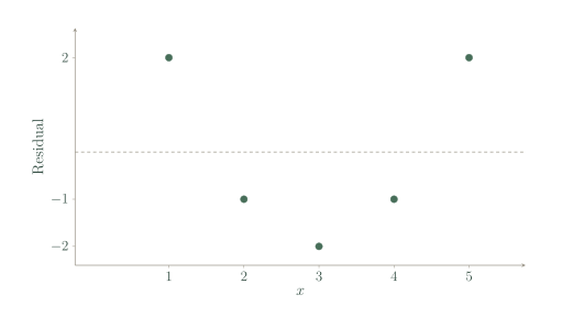
Residuals at x=1,2,3,4,5 are 2,-1,-2,-1,2. What pattern is present?
| x | Residual |
|---|---|
| 1 | 2 |
| 2 | -1 |
| 3 | -2 |
| 4 | -1 |
| 5 | 2 |
Worked solution
- 1
Read the residuals in increasing predictor order.
The predictor order reveals where overestimates and underestimates occur.
- 2
Translate the signs into model errors.
Positive residuals at both ends mean underestimation there; negative middle residuals mean overestimation in the middle.
- 3
Identify the systematic shape.
The residuals form a U-shaped pattern rather than patternless scatter. This suggests the linear model has missed curvature, so a suitable curved model should be investigated.
The linear model misses a curved relationship.
Try it yourself.
Check your understanding
Observed y=12 and predicted y=15. Find the residual.
Show answer & reasoning
-3.
Subtract in the required order: . The observation is 3 units below the prediction, so the model overestimates this observation.
Keep practising
6 worksheet questions · 18 marks
Read the questions online
- For and the observation , find the residual.3 marks
- For and the observation , find the residual.3 marks
- A residual is kg. Interpret its sign and unit.3 marks
- Residuals are ,0.6,,0.1,. Find their sum. Does a zero sum alone prove a good fit?3 marks
- Residual spread grows as increases. What feature needs investigation?3 marks
- A line was chosen by eye, not fitted by least squares. Must its residuals sum to zero?3 marks
Read the worked solutions
Equivalent correct methods earn the corresponding marks. Include units where asked.
- For and the observation , find the residual.3 marks
Predicted response is .
.
2. - For and the observation , find the residual.3 marks
Predicted response is 17.
.
. - A residual is kg. Interpret its sign and unit.3 marks
Residuals retain response units.
The observation is 4 kg below the prediction, so the model overestimates mass by 4 kg. - Residuals are ,0.6,,0.1,. Find their sum. Does a zero sum alone prove a good fit?3 marks
Add the signed residuals.
A zero sum can coexist with curvature or other unsuitable patterns.
; no. - Residual spread grows as increases. What feature needs investigation?3 marks
The fit may have non-constant error spread.
A single typical prediction error may not describe the whole range.
The variability of errors may increase with . - A line was chosen by eye, not fitted by least squares. Must its residuals sum to zero?3 marks
A freely chosen line is not constrained by that fitting condition.
No. The zero-sum property applies to the least-squares intercept fit to the same data.
Curriculum reference & lesson scope
SACE Board of South Australia
Stage 2 General Mathematics: statistical models. Original lessons and assessment practice; not an official SACE assessment.
Official curriculum source ↗