Normal probabilities and inverse-normal values | Year 12 | General Mathematics

01 / LEARN

Understand the idea.

Turn the wording into an area

Identify the shaded region before using a normal calculator. Write the desired lower tail, upper tail or interval, and standardise its boundaries using $σ$ . With $Φ (z) = P (Z < z)$ , an upper tail is $1 - Φ (z)$ and an interval is the difference of two cumulative areas.

Check that the result lies between zero and one and suits the region's size. For $n$ measurements each having event probability $p$ , the expected event count is $n p$ . Mean and standard deviation alone do not determine normal probabilities without a normal-model assumption.

\begin{aligned} P (a < X < b) & = Φ (\frac{b - μ}{σ}) \\ - Φ (\frac{a - μ}{σ}) \end{aligned}

Normal density with mean five hundred grams and standard deviation four grams. The area between 496 and 506 grams is shaded; limits and mean are marked.

Inverse normal means work from area to value

An inverse normal calculation starts with an area and finds its boundary. Convert the wording to a lower-tail proportion $p$ , calculate $z = Φ^{- 1} (p)$ , then return to original units using $x = μ + σ z$ . The highest 10% starts above the mean at lower-tail area $0.90$ .

Retain guard digits until the final cutoff and round to sensible measurement units. Check the side of the mean: an upper percentile should give a positive standardised value. In a continuous normal model, including an interval endpoint does not change its probability.

02 / WORKED EXAMPLES

See the method in action.

EXAMPLE 01

Between two masses

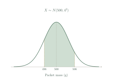
Mass X has mean 500 g and SD 4 g. Find P(496<X<506).

Worked solution

1
State the distribution assumption for the calculation.
$X \sim N (500, 4^{2})$
Use the normal-model assumption of this lesson. A mean and standard deviation alone would not determine the requested interval probability.
2
Standardise both mass limits.
$\begin{aligned} z_{lower} & = \frac{496 - 500}{4} = - 1 \\ z_{upper} & = \frac{506 - 500}{4} = 1.5 \end{aligned}$
The lower limit is one standard deviation below the mean and the upper is one and a half above it.
3
Subtract the cumulative areas.
$\begin{aligned} P (496 < X < 506) & = Φ (1.5) - Φ (- 1) \\ \approx 0.9332 - 0.1587 \\ = 0.7745 \end{aligned}$
Subtracting the area below the lower boundary from that below the upper leaves only the interval between them.
4
Interpret the probability.
$0.7745 \approx 77.45 %$
Under the normal model, about 77.45% of packet masses fall between 496 g and 506 g.

Answer

0.7745.

EXAMPLE 02

An upper cutoff

Scores are normal with mean 70 and SD 8. Find the cutoff for the highest 10%.

Worked solution

1
Convert the upper-tail wording to a lower-tail area.
$P (X > c) = 0.10 ⟹ P (X < c) = 0.90$
The cutoff for the highest 10% leaves 90% of the continuous distribution below it.
2
Find the standard normal boundary.
$z = Φ^{- 1} (0.90) \approx 1.2815516$
The positive z-value is consistent with a cutoff above the mean.
3
Convert the boundary to score units.
$\begin{aligned} c & = μ + σ z \\ = 70 + 8 (1.2815516 \dots) \\ \approx 80.25 \end{aligned}$
Using the unrounded inverse-normal value gives the stated cutoff of approximately 80.25, with about 10% of modelled scores above it.

Answer

Approximately 80.25.

03 / YOUR TURN

Try it yourself.

Check your understanding

For X normal with mean 20 and SD 2, find the median.

Show answer & reasoning

20.

The median splits the probability into equal halves. A normal distribution is symmetric about its mean, so its median is the mean, $20$ , regardless of the standard deviation.

Keep practising

6 worksheet questions · 18 marks

Open worksheet Worked solutions

Read the questions online

For $Z$ standard normal, calculate $P (Z < 1.2)$ .
3 marks
For $Z$ standard normal, calculate $P (Z > 1.2)$ .
3 marks
For $X$ with mean 50 and SD 6, find $P (44 < X < 62)$ .
3 marks
For $X$ with mean 100 and SD 12, find the 25th percentile.
3 marks
A normal quality model gives $P (pass) = 0.94$ . Out of 250 items, find the expected number passing.
3 marks
Find the upper 5% cutoff for a normal variable with mean 40 and SD 3.
3 marks

Read the worked solutions

Equivalent correct methods earn the corresponding marks. Include units where asked.

For $Z$ standard normal, calculate $P (Z < 1.2)$ .
3 marks
Use the standard normal lower-tail function at 1.2.
0.8849.
For $Z$ standard normal, calculate $P (Z > 1.2)$ .
3 marks
Use $1 - Φ (1.2)$ .
0.1151.
For $X$ with mean 50 and SD 6, find $P (44 < X < 62)$ .
3 marks
The $z$ -limits are $- 1$ and 2.
Subtract $Φ (- 1)$ from $Φ (2)$ .
0.8186.
For $X$ with mean 100 and SD 12, find the 25th percentile.
3 marks
Use $z = Φ^{- 1} (0.25)$ .
Calculate $100 + 12 z$ .
91.91.
A normal quality model gives $P (pass) = 0.94$ . Out of 250 items, find the expected number passing.
3 marks
$Expected count = 250 \times 0.94$ .
This is an expectation, not a guaranteed realised count.
235.
Find the upper 5% cutoff for a normal variable with mean 40 and SD 3.
3 marks
Top 5% means lower-tail area 0.95.
Calculate $40 + 3 Φ^{- 1} (0.95)$ .
44.93.

Checking saved progress…

Curriculum reference & lesson scope

SACE Board of South Australia

Stage 2 General Mathematics: statistical models. Original lessons and assessment practice; not an official SACE assessment.

Official curriculum source ↗

In this lesson

Understand the idea.

Turn the wording into an area

Inverse normal means work from area to value

See the method in action.

Between two masses

State the distribution assumption for the calculation.

Standardise both mass limits.

Subtract the cumulative areas.

Interpret the probability.

An upper cutoff

Convert the upper-tail wording to a lower-tail area.

Find the standard normal boundary.

Convert the boundary to score units.

Try it yourself.

Check your understanding

Keep practising