Least-squares regression | Year 12

01 / LEARN

Understand the method.

THE CORE RULE

\hat{y} = a + b x, a = \bar{y} - b \bar{x}

The line predicts $y$ from $x$ and passes through the point of sample means $(\bar{x}, \bar{y})$ .

Measure vertical prediction errors

A residual is the observed response minus the predicted response at the same $x$ . It is a vertical difference on the scatter plot.

Least squares chooses the slope and intercept that minimise the sum of squared residuals. Squaring prevents positive and negative errors cancelling.

e = y - \hat{y}

Calculate slope first, then intercept

Use centred sums, or correlation and standard deviations, to find the slope. Then substitute the two sample means to find the intercept.

Keep unrounded coefficients for calculations. Round the final prediction to a precision that suits the measurements.

\begin{aligned} b & = \frac{S_{x y}}{S_{x x}} = r \frac{s_{y}}{s_{x}} \\ a & = \bar{y} - b \bar{x} \end{aligned}

Check what the model can predict

Name the response, the explanatory variable and their units. Record the observed $x$ -range before making predictions.

Inspect the scatter plot: a calculated line is not automatically a sensible model. Curvature, clusters or influential outliers may need attention.

02 / WORKED EXAMPLES

See the method in action.

EXAMPLE 01

Calculate a fitted line

Fit $y$ on $x$ to the supplied table.

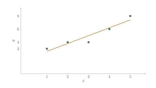
Five sage points (1,3), (2,4), (3,4), (4,6), (5,8) appear with the gold least-squares line y-hat equals 1.4 plus 1.2x, drawn from x one to five. The original labelled values and unlabelled outer padding are retained.

Paired measurements
x	y
1	3
2	4
3	4
4	6
5	8

Worked solution

1
Calculate the sample means.
$\bar{x} = 3, \bar{y} = 5$
Use all five paired rows from the supplied table.
2
Calculate the centred sums and slope.
$\begin{aligned} S_{x x} & = 4 + 1 + 0 + 1 + 4 = 10 \\ S_{x y} & = 4 + 1 + 0 + 1 + 6 = 12 \\ b & = \frac{12}{10} = 1.2 \end{aligned}$
Multiply matching deviations for $S_{x y}$ ; square the $x$ -deviations for $S_{x x}$ .
3
Find the intercept and state the model.
$\begin{aligned} a & = 5 - 1.2 (3) = 1.4 \\ \hat{y} & = 1.4 + 1.2 x \end{aligned}$
At $x = 3$ , the predicted response is $5$ , so the line passes through the point of means.

Answer

$\hat{y} = 1.4 + 1.2 x$ . The observed input range is $1 \leq x \leq 5$ .

EXAMPLE 02

Fit from summary statistics

For $\bar{x} = 10$ , $\bar{y} = 25$ , $s_{x} = 4$ , $s_{y} = 6$ and $r = 0.8$ , find the regression line.

Worked solution

1
Use correlation and the two standard deviations.
$b = 0.8 \times \frac{6}{4} = 1.2$
The response standard deviation goes in the numerator because the model predicts $y$ from $x$ .
2
Substitute the means to find the intercept.
$a = 25 - 1.2 (10) = 13$
A fitted line with an intercept passes through $(10, 25)$ .
3
Write the prediction equation.
$\hat{y} = 13 + 1.2 x$
The hat distinguishes a predicted response from an observed one.

Answer

$\hat{y} = 13 + 1.2 x$ .

03 / YOUR TURN

Try it yourself.

Calculate, explain, then apply.

CHECK 01

Use the point of means

Given $\bar{x} = 4$ , $\bar{y} = 9$ and slope $b = 2$ , find the intercept.

Show answer & reasoning

$a = 1$ .

Use $a = 9 - 2 (4) = 1$ .

Keep practising

6 worksheet questions · 18 marks

Open worksheet Worked solutions

Read the questions online

Find the line from $\bar{x} = 6, \bar{y} = 20, S_{x x} = 10$ and $S_{x y} = 25$ .
3 marks
Given $r = - 0.6, s_{x} = 5, s_{y} = 10, \bar{x} = 8$ and $\bar{y} = 30$ , find the regression line.
3 marks
A candidate line has residuals $- 2$ ,1,1. Calculate its sum of squared residuals.
3 marks
Two models have residuals $A = (- 3, 0, 3)$ and $B = (- 2, 1, 1)$ . Which has the smaller least-squares error?
3 marks
A regression line has $a = 7$ and $b = 0.5$ . Predict $y$ at $x = 12$ .
3 marks
A student rounds $b = 0.08473$ to 0.1 before predicting at $x = 900$ . Explain the risk.
3 marks

Read the worked solutions

Equivalent correct methods earn the corresponding marks. Include units where asked.

Find the line from $\bar{x} = 6, \bar{y} = 20, S_{x x} = 10$ and $S_{x y} = 25$ .
3 marks
$b = \frac{25}{10} = 2.5$ .
$a = 20 - 2.5 \times 6 = 5$ .
$\hat{y} = 5 + 2.5 x$ .
Given $r = - 0.6, s_{x} = 5, s_{y} = 10, \bar{x} = 8$ and $\bar{y} = 30$ , find the regression line.
3 marks
$b = - 0.6 \times \frac{10}{5} = - 1.2$ .
$a = 30 - (- 1.2 \times 8) = 39.6$ .
$\hat{y} = 39.6 - 1.2 x$ .
A candidate line has residuals $- 2$ ,1,1. Calculate its sum of squared residuals.
3 marks
Square each residual: 4,1,1.
Add the squares, not their signed values.
6.
Two models have residuals $A = (- 3, 0, 3)$ and $B = (- 2, 1, 1)$ . Which has the smaller least-squares error?
3 marks
A has squared sum $9 + 0 + 9 = 18$ .
B has $4 + 1 + 1 = 6$ , so B is better on this criterion.
B.
A regression line has $a = 7$ and $b = 0.5$ . Predict $y$ at $x = 12$ .
3 marks
Substitute $x = 12$ into $\hat{y} = 7 + 0.5 x$ .
$7 + 6 = 13$ .
13.
A student rounds $b = 0.08473$ to 0.1 before predicting at $x = 900$ . Explain the risk.
3 marks
A small coefficient rounding can become large after multiplication by $x$ .
Keep guard digits until the final prediction.
The slope contribution changes from 76.257 to 90, an error of 13.743.

Checking saved progress…

Curriculum reference & lesson scope

SACE Board of South Australia

Stage 2 General Mathematics: statistical models. Original lessons and assessment practice; not an official SACE assessment.

Official curriculum source ↗

In this lesson

Understand the method.

Measure vertical prediction errors

Calculate slope first, then intercept

Check what the model can predict

See the method in action.

Calculate a fitted line

Calculate the sample means.

Calculate the centred sums and slope.

Find the intercept and state the model.

Fit from summary statistics

Use correlation and the two standard deviations.

Substitute the means to find the intercept.

Write the prediction equation.

Try it yourself.

Use the point of means

Keep practising