Normal distributions | Year 12 | General Mathematics

01 / LEARN

Understand the idea.

What a normal model describes

A normal distribution is a continuous, symmetric bell-shaped probability model. Its mean $μ$ sets the centre and its standard deviation $σ > 0$ sets the spread. Here $X \sim N (μ, σ^{2})$ uses variance as the second parameter, so take its square root to find the standard deviation.

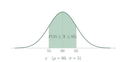
The total area under the density curve is one. Interval probabilities are areas, not curve heights. Each exact value has probability zero in this continuous model, and half the total area lies on each side of the mean.

Normal density with mean 60 and standard deviation 5, drawn from 42.5 to 77.5. The area from 55 to 65 is shaded, with dashed vertical guides at 55, 60 and 65.

Standardise and assess the approximation

Standardise using $z = \frac{x - μ}{σ}$ . A positive value is above the mean; a negative value is below it. Its magnitude is the distance from the mean measured in standard deviations, allowing comparisons on a common standard normal scale.

In a normal model, about $68 %$ , $95 %$ and $99.7 %$ lie within one, two and three standard deviations of the mean. These are approximate checks. Before applying them to real data, look for a single roughly symmetric bell-shaped group and a suitable context.

Z = \frac{X - μ}{σ} \sim N (0, 1)

02 / WORKED EXAMPLES

See the method in action.

EXAMPLE 01

Read the notation

Packet masses follow X~N(500,16) in grams. State μ and σ, and give the approximate central 95% interval.

Worked solution

1
Read the mean and variance from the stated notation.
$μ = 500 g, σ^{2} = 16 g^{2}$
In this lesson the second parameter of a normal distribution is the variance.
2
Recover the standard deviation.
$σ = \sqrt{16} = 4 g$
Standard deviation is the positive square root of variance and has the original measurement units.
3
Find two standard deviations on either side of the mean.
$\begin{aligned} μ - 2 σ & = 500 - 2 (4) = 492 g \\ μ + 2 σ & = 500 + 2 (4) = 508 g \end{aligned}$
The empirical normal rule gives an approximate central 95% interval of 492–508 g; the exact central 95% endpoints would use a different multiplier.

Answer

μ=500 g, σ=4 g; approximately 492–508 g.

EXAMPLE 02

Standardise a score

A normal score model has μ=70 and σ=8. Standardise a score of 82.

Worked solution

1
Calculate the displacement from the mean.
$x - μ = 82 - 70 = 12$
The score exceeds the mean by 12 score units.
2
Divide by the standard deviation.
$z = \frac{82 - 70}{8} = \frac{12}{8} = 1.5$
Dividing by the spread expresses the displacement in standard deviation units.
3
Interpret the standardised score.
$z = + 1.5$
The positive sign means the score is 1.5 standard deviations above the modelled mean, rather than 1.5 score units above it.

Answer

z=1.5.

03 / YOUR TURN

Try it yourself.

Check your understanding

For X~N(30,25), what is P(X<30)?

Show answer & reasoning

0.5.

The mean is $30$ and is the normal distribution's symmetry centre. Half the total area is below it, so $P (X < 30) = 0.5$ ; the single endpoint itself has probability zero.

Keep practising

6 worksheet questions · 18 marks

Open worksheet Worked solutions

Read the questions online

For $X \sim N (40, 9)$ , state the mean and standard deviation.
3 marks
A normal model has $μ = 100$ and $σ = 15$ . Standardise $x = 85$ .
3 marks
For $μ = 60$ and $σ = 5$ , give the approximate central 68% interval.
3 marks
For $μ = 60$ and $σ = 5$ , give the approximate central 99.7% interval.
3 marks
In a continuous normal model, find $P (X = μ)$ .
3 marks
A histogram has two well-separated peaks. Is a single normal model automatically justified by knowing its mean and SD?
3 marks

Read the worked solutions

Equivalent correct methods earn the corresponding marks. Include units where asked.

For $X \sim N (40, 9)$ , state the mean and standard deviation.
3 marks
The second parameter is variance 9.
Take its positive square root.
$μ = 40$ ; $σ = 3$ .
A normal model has $μ = 100$ and $σ = 15$ . Standardise $x = 85$ .
3 marks
$\frac{85 - 100}{15} = - 1$ .
$z = - 1$ .
For $μ = 60$ and $σ = 5$ , give the approximate central 68% interval.
3 marks
Use $μ \pm σ$ .
55 to 65.
For $μ = 60$ and $σ = 5$ , give the approximate central 99.7% interval.
3 marks
Use $μ \pm 3 σ$ .
45 to 75.
In a continuous normal model, find $P (X = μ)$ .
3 marks
A single point has zero interval width and area.
This does not mean values near $μ$ are unlikely.
0.
A histogram has two well-separated peaks. Is a single normal model automatically justified by knowing its mean and SD?
3 marks
Investigate distinct groups or another distribution.
No. The bimodal shape suggests that one bell-shaped model may be unsuitable.

Checking saved progress…

Curriculum reference & lesson scope

SACE Board of South Australia

Stage 2 General Mathematics: statistical models. Original lessons and assessment practice; not an official SACE assessment.

Official curriculum source ↗

In this lesson

Understand the idea.

What a normal model describes

Standardise and assess the approximation

See the method in action.

Read the notation

Read the mean and variance from the stated notation.

Recover the standard deviation.

Find two standard deviations on either side of the mean.

Standardise a score

Calculate the displacement from the mean.

Divide by the standard deviation.

Interpret the standardised score.

Try it yourself.

Check your understanding

Keep practising