Linear programming | Year 12

01 / LEARN

Understand the idea.

Organise the model before solving

Start a linear programming model by defining each variable and its units. For every resource, multiply its per-unit use by the relevant quantities, then compare the total with the available amount. Write the objective separately.

Include non-negativity, supported minimums and capacity limits. Decide whether quantities are continuous or whole numbers before solving: a solution in fractions may be meaningful for kilograms but impossible for completed vehicles.

Explain the recommendation

For a bounded feasible polygon, find and verify all vertices, evaluate the objective at each, and compare. Report the winning quantities and objective value in context. Substitute back into the resource expressions to show whether any resource remains unused.

For an unbounded region, also examine its directions extending indefinitely. It can still have a finite minimum if moving outward only increases cost. A corner comparison alone must not ignore a direction in which the objective improves without limit.

02 / WORKED EXAMPLES

See the method in action.

EXAMPLE 01

A complete production model

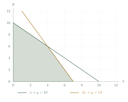
Maximise $P = 5 x + 3 y$ subject to $x, y \geq 0$ , $x + y \leq 10$ and $2 x + y \leq 14$ .

A first-quadrant grid runs from zero to twelve on both axes. The region with vertices (0,0), (7,0), (4,6), (0,10) is shaded under the supplied lines x+y=10 and 2x+y=14. No objective values are marked.

Worked solution

1
Find the feasible vertices.
$\begin{aligned} y = 0 & : x \leq 7 \\ x = 0 & : y \leq 10 \\ x + y = 10, 2 x + y = 14 & : (x, y) = (4, 6) \end{aligned}$
The origin, the tight axis bounds and the two-line intersection give $(0, 0), (7, 0), (4, 6), (0, 10)$ .
2
Evaluate the objective at every vertex.
$\begin{aligned} P (0, 0) & = 0 \\ P (7, 0) & = 35 \\ P (4, 6) & = 20 + 18 = 38 \\ P (0, 10) & = 30 \end{aligned}$
The feasible set is bounded, so a linear objective attains a maximum at one of these vertices.
3
Select the best feasible point.
$P_{max} = 38 at (x, y) = (4, 6)$
The value 38 exceeds each other corner value.
4
Check the resource use.
$4 + 6 = 10, 2 (4) + 6 = 14$
The recommended point satisfies non-negativity and uses both available resources exactly.

Answer

Maximum 38 at $(4, 6)$ .

EXAMPLE 02

A minimum-cost mix

Minimise $C = 3 x + 4 y$ subject to $x, y \geq 0$ , $x + y \geq 8$ and $x + 2 y \geq 12$ .

Worked solution

1
Find the lower boundary corners.
$\begin{aligned} y = 0 & : x \geq 12 \\ x = 0 & : y \geq 8 \\ x + y = 8, x + 2 y = 12 & : (x, y) = (4, 4) \end{aligned}$
The feasible lower boundary passes through $(12, 0), (4, 4), (0, 8)$ .
2
Compare their costs.
$\begin{aligned} C (12, 0) & = 36 \\ C (4, 4) & = 12 + 16 = 28 \\ C (0, 8) & = 32 \end{aligned}$
Along each connecting line segment, a linear cost has no value below its lower-cost endpoint.
3
Check the unbounded directions.
$\begin{aligned} C (12 + t, 0) & = 36 + 3 t \\ C (0, 8 + t) & = 32 + 4 t, t \geq 0 \end{aligned}$
Cost increases along both boundary rays; with positive coefficients, moving above the lower boundary cannot reduce it.
4
Verify and report the minimum.
$4 + 4 = 8, 4 + 2 (4) = 12, C_{min} = 28$
The point $(4, 4)$ is feasible and has the least cost among the boundary corners and rays.

Answer

Minimum 28 at $(4, 4)$ .

03 / YOUR TURN

Try it yourself.

Check your understanding

Maximise $P = 2 x + 3 y$ for $x, y \geq 0$ , $x + y \leq 5$ .

Show answer & reasoning

Maximum 15 at $(0, 5)$ .

The feasible triangle has vertices $(0, 0), (5, 0), (0, 5)$ . Their objective values are $0, 10, 15$ , so the maximum is 15 at $(0, 5)$ .

Keep practising

6 worksheet questions · 12 marks

Open worksheet Worked solutions

Read the questions online

Maximise $P = 4 x + 3 y$ for $x, y \geq 0$ , $x + y \leq 8$ , $x \leq 5$ .
2 marks
Maximise $P = 3 x + 5 y$ for $x, y \geq 0$ , $x + y \leq 9$ , $x + 2 y \leq 14$ .
2 marks
Minimise $C = 2 x + 5 y$ for $x, y \geq 0$ , $x + y \geq 6$ .
2 marks
Why has $P = x + y$ no finite maximum when only $x, y \geq 0$ is required?
2 marks
A high-profit proposal uses 18 hours when at most 16 are available. Is it acceptable?
2 marks
The optimum for $P = 5 x + 3 y$ is $(4, 6)$ . If $P$ is in hundreds of dollars, interpret the result.
2 marks

Read the worked solutions

Equivalent correct methods earn the corresponding marks. Include units where asked.

Maximise $P = 4 x + 3 y$ for $x, y \geq 0$ , $x + y \leq 8$ , $x \leq 5$ .
2 marks
The vertices are $(0, 0), (5, 0), (5, 3), (0, 8)$ .
Their values are 0,20,29,24.
Maximum 29 at $(5, 3)$ .
Maximise $P = 3 x + 5 y$ for $x, y \geq 0$ , $x + y \leq 9$ , $x + 2 y \leq 14$ .
2 marks
Vertices are $(0, 0), (9, 0), (4, 5), (0, 7)$ .
Values are 0,27,37,35.
Maximum 37 at $(4, 5)$ .
Minimise $C = 2 x + 5 y$ for $x, y \geq 0$ , $x + y \geq 6$ .
2 marks
Rewrite the objective as $C = 2 (x + y) + 3 y$ .
Since $x + y \geq 6$ and $y \geq 0$ , $C \geq 12$ ; $(6, 0)$ attains that bound.
Minimum 12 at $(6, 0)$ .
Why has $P = x + y$ no finite maximum when only $x, y \geq 0$ is required?
2 marks
Feasible points $(t, 0)$ have arbitrarily large objective $t$ .
It is unbounded above.
A high-profit proposal uses 18 hours when at most 16 are available. Is it acceptable?
2 marks
An infeasible decision is excluded regardless of its profit.
No.
The optimum for $P = 5 x + 3 y$ is $(4, 6)$ . If $P$ is in hundreds of dollars, interpret the result.
2 marks
$P = 38$ hundreds, so multiply by 100.
AUD 3,800.

Checking saved progress…

Curriculum reference & lesson scope

SACE Board of South Australia

Stage 2 General Mathematics: Modelling with Linear Relationships, a compulsory school-assessed topic. The external examination scope differs from the full course.

Official curriculum source ↗

In this lesson

Understand the idea.

Organise the model before solving

Explain the recommendation

See the method in action.

A complete production model

Find the feasible vertices.

Evaluate the objective at every vertex.

Select the best feasible point.

Check the resource use.

A minimum-cost mix

Find the lower boundary corners.

Compare their costs.

Check the unbounded directions.

Verify and report the minimum.

Try it yourself.

Check your understanding

Keep practising